English is promiscuous. If it likes a word or expression, it steals it. "Not invented here" is no objection. Official French is the opposite. The Académie Française resists the contamination of the purity of the language with anglicisms such as "streamer," which the academicians insist should be expressed as joueur-animateur en direct. Language purists exist in programming as well.
It's unlikely that any single language can be the best at everything, but for serious software development it can be impractical to mix and match.
Fortunately, in my world of casual, ad-hoc programming, I have that luxury. And I am now using a language, Julia. that makes it possible to build contraptions that draw from work I've done in other languages. One of those languages is R, the open-source successor to S, which was the product of some heavyweight statisticians at Bell Labs working just down the hall from the immortals who gave us Unix and C. R is an interactive language designed with functional use in mind, y = f(x) where you express your problem in terms of library functions operating on an object and parameters. It's a very natural way to express math problems. The heavy lifting is done behind the scenes by well exercised libraries in Fortran and C. It comes packaged with all the standard undergradsuate level textbook statistical functions and packages for stuff found in graduate level texts are available from the vast trove of contributed packages. Anything you can't find is probably above your pay grade.
R does, however, suffer from a lack of beauty and elegance in its offerings as a scripting language. It's turing complete, so it can do anything, but it does so gracelessly. After using it almost exclusively for 15 years, I took up Julia. I've been happy. But sometimes I need a tool from R for which there is nothing on offer in Julia.
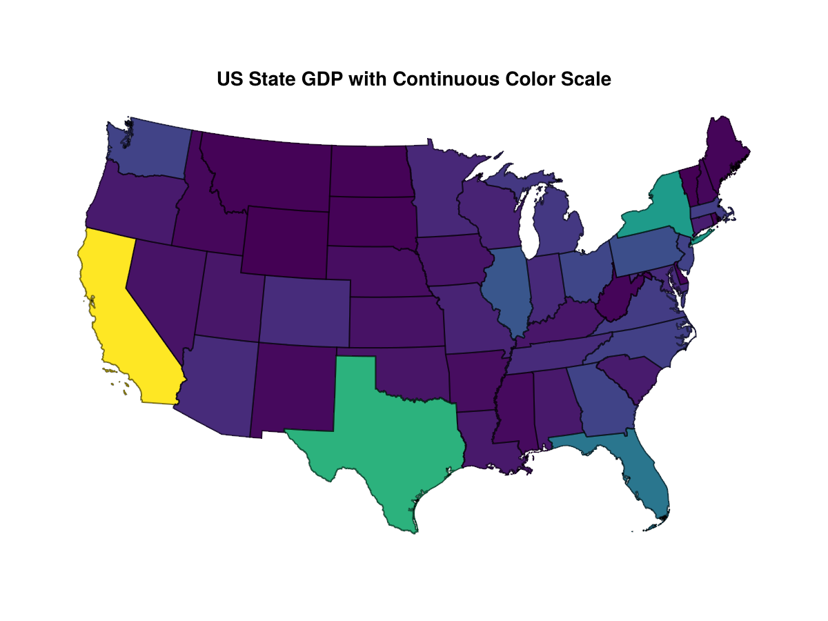
Take thematic maps. A map of the states colored according to gross domestic product, say, will be difficult to read if a continuous scale is used.
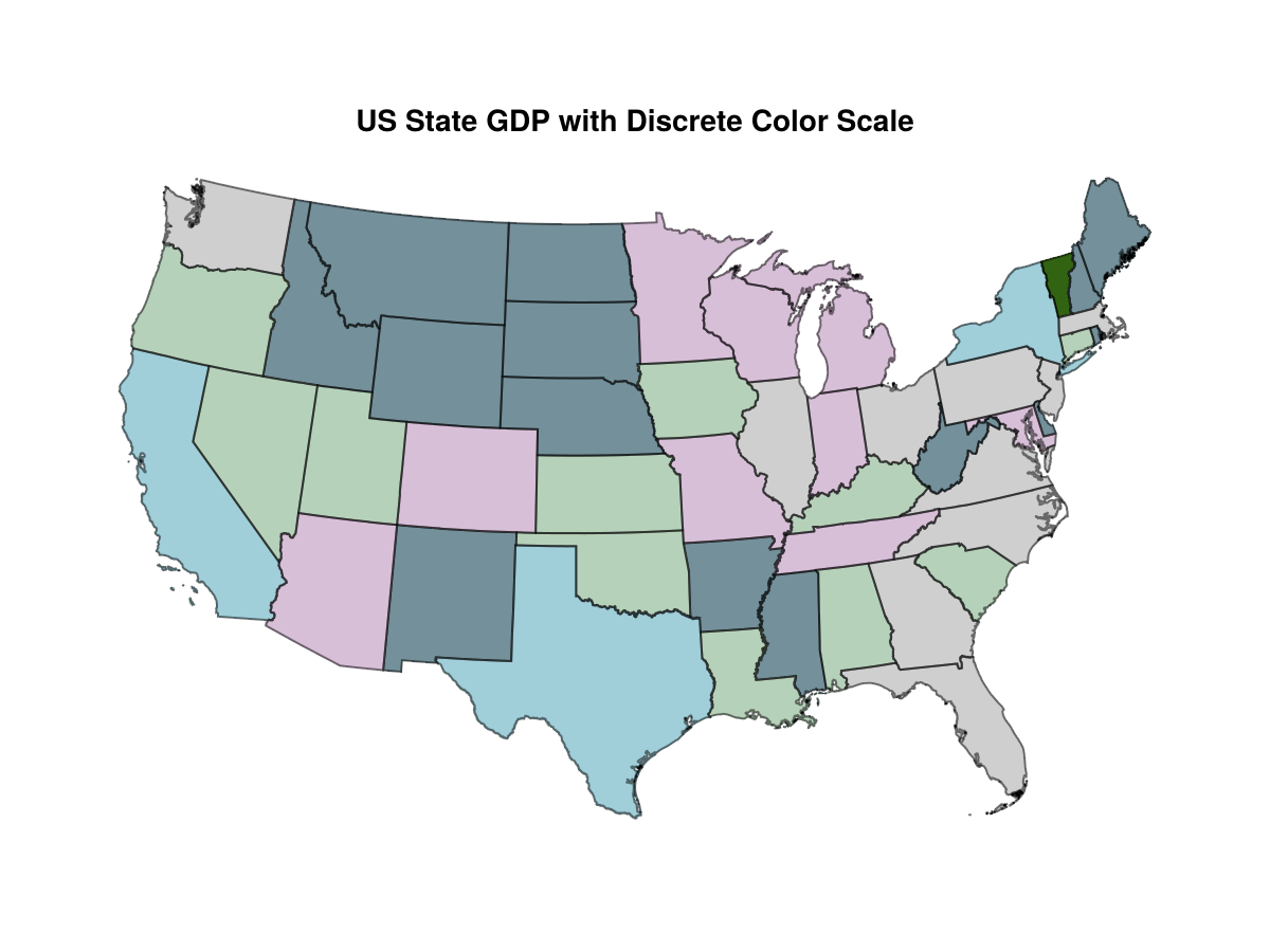
 A discrete color scale allows the differences among the smaller states more clearly to be seen.
 This requires partitioning the data somehow. The R library classInt provides options to do this, and I've found nothing similar in Julia. Here's how this works.
using DataFrames
using RCall

SETUP_COMPLETE = [false]

function setup_r_environment()
    if SETUP_COMPLETE[]
        return nothing
    end

R"""
    # Set the correct ARM64 path for R explicitly
    .libPaths(c("/Library/Frameworks/R.framework/Versions/Current/Resources/library"))
    required_packages <- c("classInt")

    # R function to install missing packages
    install_if_missing <- function(pkg) {
        if (!require(pkg, character.only = TRUE)) {
            install.packages(pkg, repos  = "https://cran.rstudio.com/")
        }
    }

    # Install missing packages
    invisible(sapply(required_packages, install_if_missing))

    # Verify installations
    installed <- sapply(required_packages, require, character.only = TRUE)
    print(data.frame(
        Package   = required_packages,
        Installed = installed
    ))
"""
    SETUP_COMPLETE[] = true
    return nothing
end

setup_r_environment()

function get_breaks(DF::DataFrame, col_no::Int)
    @rput DF
    @rput col_no
    R"""
    library(classInt)
    x   = DF[,col_no]
    breaks  <- list(
        fisher      = classIntervals(x, n=5, style="fisher"),
        jenks       = classIntervals(x, n=5, style="jenks"),
        kmeans      = classIntervals(x, n=5, style="kmeans"),
        maximum     = classIntervals(x, style="maximum"),
        pretty      = classIntervals(x, n=5, style="pretty"),
        quantile    = classIntervals(x, n=5, style="quantile"),
        sd          = classIntervals(x, n=5, style="sd")
    )
    """
end

df = DataFrame(gdp = [1.10323705e11, 5.7275094e10, 3.248656553e12, 2.24418023e11, 2.45354674e11, 6.78201178e11, 1.42860555e11, 7.99228807e11, 3.48487426e11, 4.37056036e11, 2.25459425e11, 2.07923341e11, 4.22087716e11, 4.0210781e10, 1.791210722e12, 4.04290315e11, 1.83795569e11, 9.5897911e10, 1.95405599e11, 8.85651322e11, 3.5236566e10, 3.90907909e11, 2.02051377e11, 2.62298502e11, 9.3466707e10, 7.8014386e10, 1.4602426e11, 2.86628442e11, 5.54256192e11, 6.15504521e11, 1.292787615e12, 6.6388854e11, 6.0348597e10, 4.22866291e11, 7.5195388e10, 6.3277041e10, 5.7373329e10, 4.22399581e11, 1.45019622e11, 6.77238047e11, 2.097090405e12, 7.09816649e11, 3.44570759e11, 2.61951538e11, 1.19548365e11, 6.38067296e11, 5.97597103e11, 8.0798157e10, 2.48615513e11
This will return an object with a selection of ways to partition the vector:
julia> println(get_breaks(df,1))
RObject{VecSxp}
$fisher
style: fisher
  one of 194,580 possible partitions of this variable into 5 classes
  [35236566000,2.35407e+11)  [2.35407e+11,495656114000)
                         22                          13
[495656114000,1.089219e+12) [1.089219e+12,2.672873e+12)
                         10                           3
[2.672873e+12,3.248657e+12]
                          1

$jenks
style: jenks
  one of 194,580 possible partitions of this variable into 5 classes
[35236566000,225459425000] (225459425000,4.37056e+11]
                        22                         13
(4.37056e+11,885651322000] (885651322000,2.09709e+12]
                        10                          3
(2.09709e+12,3.248657e+12]
                         1

$kmeans
style: kmeans
  one of 194,580 possible partitions of this variable into 5 classes
 [35236566000,164909914500) [164909914500,315599600500)
                         16                          11
[315599600500,575926647500) [575926647500,1.541999e+12)
                          9                          10
[1.541999e+12,3.248657e+12]
                          3

$maximum
style: maximum
  one of 12,271,512 possible partitions of this variable into 7 classes
 [35236566000,495656114000) [495656114000,754522728000)
                         35                           8
[754522728000,1.089219e+12) [1.089219e+12,1.541999e+12)
                          2                           1
[1.541999e+12,1.944151e+12) [1.944151e+12,2.672873e+12)
                          1                           1
[2.672873e+12,3.248657e+12]
                          1

$pretty
style: pretty
  one of 12,271,512 possible partitions of this variable into 7 classes
      [0,5e+11)   [5e+11,1e+12) [1e+12,1.5e+12) [1.5e+12,2e+12) [2e+12,2.5e+12)
             35              10               1               1               1
[2.5e+12,3e+12) [3e+12,3.5e+12]
              0               1

$quantile
style: quantile
  one of 194,580 possible partitions of this variable into 5 classes
  [35236566000,94925429400)  [94925429400,211222277400)
                         10                          10
[211222277400,382423812400) [382423812400,648395793600)
                          9                          10
[648395793600,3.248657e+12]
                         10

$sd
style: sd
  one of 1,712,304 possible partitions of this variable into 6 classes
[-1.27016e+11,456870070408) [456870070408,1.040756e+12)
                         35                          10
[1.040756e+12,1.624642e+12) [1.624642e+12,2.208528e+12)
                          1                           2
[2.208528e+12,2.792414e+12)   [2.792414e+12,3.3763e+12]
                          0                           1
To retrieve one
breaks=get_breaks(df2,2)
kbreaks = rcopy(breaks[3])
breaks = convert(Vector{Float64}, kbreaks[:brks])
The tricky part is setting the environment, which is the purpose of function. There's native support for C and Fortran and packages for Python, MATLAB and Java.